4.4.2 - How to determine them?

Qualitative and quantitative method for estimating uncertainties of a Bilan Carbone®.

Source: Freepik

Uncertainties within a Bilan Carbone® take two different forms. The first is qualitative, that is to say that characteristics are defined for the activity data and the emission factors, then rated qualitatively. The second is quantitative, stems from the qualitative information and leads to the determination of a 95% confidence interval.

Reporting formats

Taking uncertainties into account results in three different but correlated forms of results:

1. A qualitative uncertainty on GHG emissions, ranging from "Very high" to "Very low"

2. A 95% confidence interval, i.e. an interval [Lower Bound; Upper Bound] within which the result has a 95% chance of lying

3. A percentage value, which means that the result is potentially % higher than its value:

These three forms of results are complementary and allow uncertainties to be reported to audiences with different levels of understanding of these issues.

Qualitative determination

The qualitative determination of uncertainties for an emission source involves completing two matrices, one for the emission factor and the other for the activity data. To fill in these two matrices, the organization must assign a quality rating (Very good, Good, Average, Poor, Very poor) to each of the five characteristics of the activity data or the emission factor. The meaning of the different characteristics is detailed below.

Characteristic	Quality
Technical representativeness	Very good
Geographical representativeness	Good
Temporal representativeness	Average
Completeness	Poor
Reliability	Very poor

The five characteristics used are as follows:

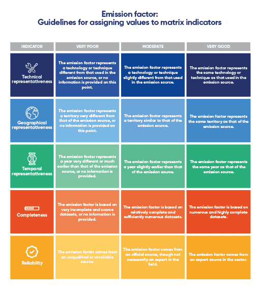
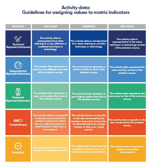
• Technical representativeness: This characteristic assesses whether the value is truly representative of the current state of techniques and technologies used. EF: Assesses whether technological advances have occurred since the emission factor was created. AD: Assesses whether the activity data comes from a different or obsolete technology.

• Geographical representativeness: This characteristic assesses whether the value is well adapted to the geographic location of the emission source. EF: Assesses whether the emission factor applies to a territory different from that of the emission source. AD: Assesses whether the activity data comes from another territory.

• Temporal representativeness: This characteristic assesses whether the value is up to date for the emission source. EF: Assesses whether the emission factor is sufficiently up to date, whether its validity period has been exceeded, or whether changes have occurred since the emission factor was created. AD: Assesses whether the activity data used comes from a different year than the year in which the assessment was carried out.

• Completeness: This characteristic assesses whether the value is statistically representative of the emission source. EF: Assesses whether the emission factor is developed from a representative dataset. AD: Assesses whether the activity data comes from statistical averages or extrapolations based on an insufficient number of data points.

• Reliability: This characteristic determines whether the method of collecting the activity data and the source from which the emission factor originates are reliable. EF: Assesses whether the emission factor comes from an unqualified or unreliable source. AD: Assesses whether the activity data is based on a rough or even speculative estimate rather than a precise measurement.

For an emission factor:

If the emission factor (EF) comes from a database that uses uncertainties, the matrix must be reviewed or completed based on the information from the database.

🔎 For the Base Empreinte®, for example, users can directly reuse the ratings associated with the EF characteristics from the database. These ratings assess the EF's ability to represent what it claims to be.

However, it may be that the organization uses an emission factor that is not entirely suited to the emission source considered. Thus, for organizations wishing to be more precise in their consideration of uncertainties, it may be relevant to adjust and reassess the ratings of the various characteristics originating from databases.

Example: The emission factor for a Spanish orange comes from a very high quality LCA, and all its ratings show "Very good". An organization that would use this emission factor for oranges from another country should ideally downgrade the rating associated with the "Geographical representativeness" characteristic.

If the emission factor does not come from a database using uncertainties, the matrix must be established from the documentation provided on the EF. If no documentation is available, the ratings associated with the EF in the matrix should be low.

⏳[WIP] A practical example of completeness (qualitative and quantitative) of the uncertainty will be available at the end of the experimentation phase, in the appendix.

Guidance for completing the matrix for an emission factor is provided below.

Figure 4.4.2 - 1: Emission factor: guidelines for assigning a value to the matrix indicators

For an activity data:

For activity data (AD), the organization must assign a rating to the activity data used.

Example: The organization's data is a number of kWh taken from the twelve invoices associated with the chosen temporal boundary. The organization assigns the rating "Very good" to this activity data.

However, for organizations wishing to be more precise in their consideration of uncertainties, it is possible, as for emission factors, to assign a rating to each of the five characteristics of the matrix.

⏳[WIP] A practical example of completeness (qualitative and quantitative) of the uncertainty will be available at the end of the experimentation phase, in the appendix.

🔎 Completed uncertainty matrices for standard collection methods will soon be available on the General Carbon Plan.

Guidance for completing the matrix for activity data is provided below.

Figure 4.4.2 - 2: Activity data: guidelines for assigning a value to the matrix indicators

Quantitative determination

The quantitative determination of uncertainties does not require any additional effort from the organization. Bilan Carbone® tools use the qualitative determination of uncertainties to automatically arrive at this quantitative determination. For this quantitative approach, it is assumed that the distribution laws of uncertainties are log-normal.

The matrices obtained via the qualitative determination serve as the basis for the quantitative determination. Coefficients are associated with each quality for each characteristic according to the matrix below:

Characteristic	Rating	Coefficient (Ecoinvent 1)
Technical representativeness	Very poor Poor Average Good Very good	U1 = 2.00 U1 = 1.50 U1 = 1.20 U1 = 1.10* U1 = 1.00 *Coefficient assigned by the ABC
Geographical representativeness	Very poor Poor Average Good Very good	U2 = 1.10 U2 = 1.05* U2 = 1.02 U2 = 1.01 U2 = 1.00 *Coefficient assigned by the ABC
Temporal representativeness	Very poor Poor Average Good Very good	U3 = 1.50 U3 = 1.20 U3 = 1.10 U3 = 1.03 U3 = 1.00
Completeness	Very poor Poor Average Good Very good	U4 = 1.20 U4 = 1.10 U4 = 1.05 U4 = 1.02 U4 = 1.00
Reliability	Very poor Poor Average Good Very good	U5 = 1.50 U5 = 1.20 U5 = 1.10 U5 = 1.05 U5 = 1.00

The geometric standard deviations (GSD) associated with the activity data and the emission factor are then calculated using the following formula:

Calculation of the GSD for an emission factor or an activity data

These two geometric standard deviations are then combined to obtain a standard deviation for the emission source, using the following formula:

Calculation of the GSD for an emission source

Using this geometric standard deviation, the organization obtains the 95% confidence interval for the emission source, which is as follows:

Confidence interval

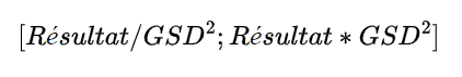
The lower value of this interval is called the "Lower Bound", and the upper value is called the "Upper Bound". It is then possible to propagate these uncertainties associated with the different emission sources to obtain uncertainties for a sub-category of emissions, an emission category, or for the entire assessment.

For a given emission source, its sensitivity is defined as its weight in the total of the assessment. Let E1 be the value of an emission source and T the total value of the assessment, the sensitivity S1 of the emission source E1 is:

Sensitivity calculation

Let E1 and E2 be the values of two emission sources, S1 and S2 their respective sensitivities and GSD(E1) and GSD(E2) their respective geometric standard deviations, the geometric standard deviation on E1 + E2 is:

GSD propagation formula.

The 95% confidence interval is then obtained using the same method as previously.

⏳[WIP] A practical example of completeness (qualitative and quantitative) of the uncertainty will be available at the end of the experimentation phase, in the appendix.

Requirements related to uncertainties

Here are different requirements to be met in terms of taking uncertainties into account for each of the 3 maturity levels.

Initial Level: criterion M1

The organization must qualify and quantify the uncertainties for all direct emissions and significant indirect emissions of the Bilan Carbone® (as a reminder, this represents at least 80% of emissions).

The qualitative determination of uncertainty can be carried out:

• by assigning a single quality rating (Very good, Good, Average, Poor, Very poor) to each activity data concerned. This overall rating is therefore representative and consistent with all 5 characteristics.

• by using as is the ratings of emission factors from databases.

The quantitative determination of uncertainty is automatically calculated from the qualitative determination.

Standard Level: criterion M2

The organization must qualify and quantify the uncertainties for all direct emissions and significant indirect emissions of the Bilan Carbone® (as a reminder, this represents at least 80% of emissions).

The qualitative determination of uncertainty can be carried out:

• by assigning a single quality rating (Very good, Good, Average, Poor, Very poor) to each activity data concerned. It is however recommended to assign a rating to each of the 5 characteristics (technical, geographical, temporal representativeness, completeness and reliability), i.e. 5 ratings for each activity data responsible for the most significant of the assessment.

• emissions, by using as is the ratings of emission factors from databases. It is however recommended to adjust these ratings when the effective use is not exactly within the scope of application intended by the database.

The quantitative determination of uncertainty is automatically calculated from the qualitative determination.

Advanced Level: criterion M3

The organization must qualify and quantify the uncertainties for all emissions in the Bilan Carbone®.

The organization must systematically use the five characteristics for activity data and modify the ratings assigned to emission factors by databases when this is relevant.

The qualitative determination of uncertainty must systematically be carried out:

• by assigning a quality rating (Very good, Good, Average, Poor, Very poor) to each of the 5 characteristics (technical, geographical, temporal representativeness, completeness and reliability), for each activity data used.

• by adjusting the ratings of emission factors from databases, when necessary (when the effective use is not exactly within the scope of application intended by the database).

The quantitative determination of uncertainty is automatically calculated from the qualitative determination.

---

Do you have a question about understanding? Consult the FAQ. The method is living and therefore likely to evolve (clarifications, additions): find the track of changes here.